Abstract : Description and photos of the e-beam system for field mapping in UST_1 . The expected magnetic surfaces as seen by the camera are calculated and shown. The power of the e-beam and the emittance of the phosphor screen is roughly calculated. The movement of the rod and other details are outlined.
Content :
* General description of the elements
* e-Beam (Structural description.
Background subtraction. Filament)
* CCD Camera
* Expected magnetic surfaces
* Calculations and control of the e-beam
(e-beam power , Emittance.
Rod movement. Camera process.
nº of toroidal turns)
* Acknowledgments
The fluorescent method will be used to visualise the magnetic surfaces. The information from [1] and [2] is studied as a guide for the system in UST_1.
I received kind explanations from Xabier Sarasola about some further details of the e-beam and fluorescent screen in the CNT system. Even a more simplified and low cost field mapping experiment is pursued here.
General description of the elements
The general aspect of the system is shown in Figure 1.
P15 phosphor screen is planned. One UK supplier sells P15 phosphor in relatively small quantities (100gr) at a moderate price. Perhaps a free 5gr sample is supplied. P15 phosphor seems practically identical to P24 phosphor which was used in CNT and in HSX. In one reference P15 is even more recommended for very low electron energy.
A movable rod and perhaps a "mesh" of tiny rods will be utilised here. A mesh with 95% transparency was used in HSX filed mapping. A rod is preferred in CNT and an elliptical wire is taken in WEGA.
e-Beam
The e-beam is made in-site to lower costs. Taking some ideas from the CNT e-beam a radical reduction in the number of pieces is carried out.
Structural description
The front of a halogen light bulb is cut and the bulb acts simultaneously as an electron source chamber and supporting structure. See Photo 1. The two pins of the bulb are silver soldered to copper rods. Two copper rods acts as current carrying elements and supporting elements. A brass cap with a 0.75mm diameter central hole is fitted on the light bulb to accelerate the electrons. It will avoid excessive background light which will difficult the vision. Finally the 3 pins (one is superfluous because the chamber must be grounded) are connected to the fedthrough.
50eV to 150eV electrons are planned.
Background subtraction
The e-beam will be activated intermittently with ON cycle of about 1 second and OFF cycle 1 second. This is intended to easy the subtraction of the background light from the source light. Some experiments use selective filters to block the bulb-light source but no filter is planned.
Filament
Barium oxides and other materials can be obtained from vacuum tubes and from companies like Kimball Physics Inc. (at higher prices). However BaO emitters are not suited for this application because it degrades at medium vacuum pressures. One important problem in UST_1 is the outgassing and consequently the difficult to reach high vacuum. Tungsten filament will be used in the first try.
CCD Camera
A low cost Unibrain firewire camera is used. These cameras are well known by Cristobal Belles who has developed an AI system for the cameras and he will help in the development. The cameras have an undetermined sensibility but it can be supposed in the range around 10 lux min. The maximum shutter is 1/30, not the best for this application, but perhaps enough according to some rough calculations below. A high sensibility photographic film or digital camera will be used if the first try is insufficient.
Expected magnetic surfaces
The image is taken from a point of view that form 105º with the projection plane. Instead of calculating the real shape of the surfaces by deformation of the image taken by the camera, here the theoretical magnetic surfaces are deformed when "observed" in 3D from the point of view where the real camera is installed. This method is easier if you do not have a suitable code to deform images. The ports were positioned to have an angle of vision similar to 90º but 105º was the best possible choice. The objective will have 30' aperture but at the beginning one of 61' is used.
The expected magnetic surfaces viewed from the point of view of the camera on the plane Toroidal angle =0º is shown in Graph 3. The plan view (perpendicular to the poloidal plane, viewed from infinite) is shown in Graph 2. A slight deformation is observed in Graph 3.
Calculations and control of the e-beam
e-beam power
15 W is the power of the halogen light bulb. The filament will have a minimum of 0.1cm2 of emission surface. At 2500K the max current density emitted from the filament is 0.26 A/cm2. At 2200K it is only 0.01 A/cm2. An adjustable power supply, 12V DC, will be used to roughly regulate the emitting power. Considering typically 2500K and an efficiency of 5% in the extraction of electrons through the 0.75mm diameter frontal acceleration hole the e-beam current will be ~1 mA . 5% is similar to the CNT e-beam obtained from some approximate calculations.
Taken an efficiency of the P15 phosphor = 7 lumen/W , reducing to 50% due to low quality coating on the rod, it results ~3lumen/W.
Power of the e-beam at 50eV =~ 0.05W.
e-beam section =~ 1mm2
Emittance
The total luminous flux from the phosphor is 0.15 lumen.
1/2 of the flux is lost in the back of the phosphor and additionally 50% might be lost. ~0.03 lumen are emitted from 1mm2 of surface. Emittance will be 37000 lux if the rod is fixed. However the phosphor is saturated far before such value. The emission power will be regulated varying the T of the filament.
Rod movement
Supposing a 1/10s shutter for the camera and 1/10 frames/s , the best option is to move a coated rod of 1mm diameter at a speed of 1cm/s so to minimise the effect of the background light . In this case it results 3700 lux.
The values of emittance are very high because the e-beam is thin.
Camera process
The camera should have long integrating time, but this low cost camera has no this possibility. Cameras 10 times more expensive, of the order of 1000€, have this option. Here the frames during about 4 seconds (a complete sweep of the poloidal section) will be added to obtain the whole magnetic surface. In this method each frame will have different individual points. The frames will be filtered to reduce background effect.
nº of toroidal turns
Another issue is the relative big size of the e-beam in relation to the size of the magnetic surfaces. It will stop most of the returning e-beams after ~3 or 10 turns depending on the particular magnetic surface. One solution, not easy, is the reduction of the size of the e-beam. With 10 turns only an outline of the surfaces will be obtained. Another solution is to simulate with SIMPIMF the best surfaces to be represented considering the present limitation.
Acknowledgments
I thank the detailed explanations from Xabier Sarasola (CIEMAT) about the e-beam and the type and use of phosphors in CNT.
References
[1] "Field line mapping results in the CNT stellarator" X. Sarasola , T. Sunn Pedersen at al.
[2] "Initial Results of Magnetic Surface Mapping in the WEGA Stellarator" M. Otte, J. Lingertat
Figure 1 . Field line mapping experimental setup
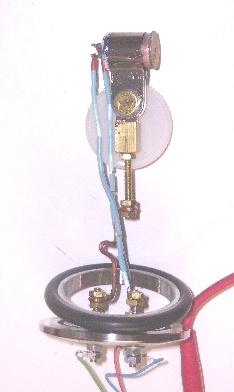
Photo 3 . Added on 29-07-06 . New version of the e-gun. The internal part is very similar to the old model (Photo 2) but the enclosure and the support has been improved. It can be moved ~15mm from the exterior of the vessel.
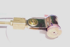
Photo 4 . Added on 29-07-06 . Detail of the new version of e-gun
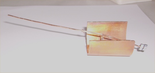
Photo 5 . Added on 29-07-06 . The movable fluorescent rod was finally designed as an oscillating rod.
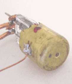
Photo 1 . Very low cost e-beam
Photo 2 . Exploded view of the e-beam.
Graph 2 . Plan view of the expected magnetic surfaces for the built design.
Graph 3 . View from the point of view of the camera of the expected magnetic surfaces. Slight deformation occurs.
Graph 4 . Plan view of some magentic islands
Date of publication 08-05-2006. Two photos added on 29-07-06