Abstract : A first optimization of the confinement and coils for UST_1 is carried out. Stellarators with the same size and winding surfaces are compared using SimPIMF v2.0. In this simulations only rotational transform, magnetic ripple and proportion of trapped particles are optimized. Averaged drifts are not taken into account. The objective is to know the features of each alternative together with the engineering constrains.
Process of optimization
Here the traditional approach for optimization is followed [1] .
The size of the device is already defined and HF coils are chosen to be external while TF coils are internal. This particular location of coils, not common, is taken due to engineering advantages. The size of the device depends on the available standard tubes and materials and cannot be optimized.
SimPIMF v2.0 code, input of data, output and process is partly described in [2]
Specifications of the device
The aim is to obtain a last closed surface with Iota = 0.33 . Some time ago a flat profile of Iota was considered, style W7-X, but it is not clear if it is possible in a classical stellartor. As a result Iota is now more variable and finally it will depend on the available electrical power for the HF coils. In a first phase Iota=0.15 is more realistic because of the limitation of electrical power. The issues related to Iota are discussed in [3].
|B| was decided equal to 0.1T at first but later
|B| ~ 0.07T, similar to WEGA stellarator, seemed a good choice to allow the
use of standard devices for microwave heating. Here |B| is around 0.1T on
the axis.
From |B| ~ Bt and SimPIMF, TF current is set to be 4700A-turns in each of
the 10 TF coils (for other number then a simple recalculation)
A set of intervals for the input parameters to define the coils is
established:
Usually 6 points are taken in the next intervals:
A) Pitch 1 : [-0.1, 0.1] m
B) Pitch 2 : [-0.05 , 0.05] m
C) Pitch 3 : not considered.
D) HF current : depending on m=3,4,5 : [1000, 10000] A
E) Position of the try for the last closed surface [mag. axis+0.010 , mag.
axis+0.030] m
Position of the magnetic axis
The position of the magnetic axis is manually obtained by trying and observation of the graphical representation. It takes 2 or 3 steps. On the coordinate axis X the radius of the magnetic axis is :
R_axis= 0.111 for m=3
R_axis= 0.106 for m=4
R_axis= 0.107 for m=5
(An error +-0.5mm can be considered)
HF current and Iota
E) is a constant in a first run and the code obtains HF for Iota = 0.32. Iota slightly depends on the pitch but a value is fixed as a start for new runs.
The results are :
HF current= 4200A-turns for m=3
HF current= 6800A-turns for m=4
HF current= 10000A-turns for m=5
Optimization of magnetic ripple and plasma size
Given HF current a new run varies A) B) E) and try to maximise simultaneously the magnetic ripple at each position of the particle which is equivalent to the last closed surface we are trying to maximise. Particles that are out of the magnetic boundaries are not considered (they escape from the system). Consequently there is a maximum value of X (birth of particle) with a stable orbit for each configuration of coils (36 configurations).
The maximum X coordinates with an acceptable ripple are:
| m | Loop | Pitch 1 | Pitch 2 | Iota | Ripple | Max X | Plasma Rad. | |
| H | 3 | 98 | -0.02 | 0.06 | 0.29 | 0.196 | 0.134 | 23 |
| I | 3 | 158 | 0.06 | -0.02 | 0.29 | 0.228 | 0.134 | 23 |
| J | 4 | 134 | 0.02 | 0.03 | 0.35 | 0.159 | 0.127 | 21 |
| K | 4 | 68 | -0.06 | 0.05 | 0.29 | 0.157 | 0.127 | 21 |
| L | 5 | 129 | 0.02 | 0.01 | 0.36 | 0.173 | 0.127 | 20 |
| M | 5 | 128 | 0.06 | 0.01 | 0.38 | 0.154 | 0.122 | 15 |
Some few configurations with higher "Max. X" but excesive ripple are not shown.
The code chooses a best option, but manually some other acceptable alternatives are found. Sometimes what is the best option for the code, which depends on some weighting factors, is not exactly the final election. This could be improved.
The last is only a rough calculation to decide about the best m=3,
4, 5 stellarator with respect to the parameters of optimization. A finer run
should be done later.
Proportion of trapped particles
A new run is done being A) and B) the only paramenters and the
switch for an additional plasma simulation is set to ON.
In this case 600 electrons in each of the 36 coil configurations is
run. 'D' simulation [2] is chosen. However it seems that a kind of Poincare
simulation including the energy balance and avoiding the drift equations
could be used [4]. The last method is faster. It took 5 hours with ‘D’
simulation.
The particles are thrown randomly in a toroidal volume of radius =
5mm . There is a limit to avoid throwing particles outside the plasma due to
the shaped volume of the plasma. A value of 10mm would have been better so
the new finer calculation will take this value.
The distribution of energy is uniform (not maxwellian yet), taking
the most probable energy of the maxwellian distribution at T=10eV.
Results:
The mean value of the proportion of trapped particles for the 36
coil configurations was :
In m=3 case was calculated and result 30.1% .
For m=4 is roughly 22% .
No values for m=5
| m | Pitch 1 | Pitch 2 | Ripple | % trapped | |
| H1 | 3 | -0.02 | 0.06 | 0.131 | 31.6 |
| H2 | 3 | -0.02 | 0.06 | 0.131 | 28.8 |
| H3 | 3 | -0.02 | 0.06 | 0.131 | 29.5 |
| H4 | 3 | -0.06 | 0.05 | 0.131 | 27.0 |
| J1 | 4 | 0.02 | 0.03 | 0.106 | 20.0 |
| J2 | 4 | 0.02 | 0.03 | 0.106 | 21.6 |
| J3 | 4 | 0.02 | 0.03 | 0.106 | 22.0 |
The ripple is smaller here than before because it is calculated at axis+10mm.
The proportion of trapped particles varies because only 600 particles are simulated. The deviation reflects the magnitude of the error.
The values are comparable with the ones shown in [4] Fig 6 and this is one data that help to verify the correction of the SimPIMF code . More particular and accurate tests are necessary.
Conclusions
Perhaps HF current is too high for this amateur
stellarator in the m=5 case, more when an important part of the total cost
of the device will be the power supplies. W7-X , W7-AS and CTH are examples
of m=5 stellarators. In [1] there is a comparison of plasma instabilities
(resistive interchange modes and ballowing modes) between m = 4, 5 , 6. m=5
was chosen there. Ripple and supposedly % of trapped particles have the
lowest values, but not far from the m=4 case. The copper vacuum vessel is a
little more capable for m=5 symmetry because it is formed by 5 elbows.
Case m=4 seems a middle point: moderate
HF current that seem achievable, low ripple similar to the best m=5 case and
moderate proportion of trapped particles. TJ-II (heliac) and MHH are cases
where m=4 was selected.
m=3 case has low HF current but this
factor is less important for 4200A-turns. Ripple and proportion of trapped
particles are high. NCSX is an example m=3 and it seems that the confinement
of trapped particles will be good [5]. However this is a very advanced
modular stellarator with all kind of optimizations.
In Graph 1 a perspective of the magnetic surface (cyan) for m=5 and the magnetic axis (yellow) is shown
A filamentary vision of the m=5 stellarator is displayed in Graph 2 and the ground plan in Graph 3.
The case m=3 in Graph 4 containing the magnetic axis in yellow.
Stellarator m=4 in Graph 5.
Currently the option m=4 seems the best.
The engineering constrains will help the final decision.
Further developments
The selected case will be further optimised.
References
[1] "Physics and engineering design for wendelstein 7-X" Craig Beidler, G. Grieger , et al. Fusion Tech. 1989
[2] "SimPIMF v2.0 code in JAVA for simulation and optimization of coils" , Vicente M. Queral . See “Past R&D" in this web
[3] "Optimum Iota Profiles" , Vicente M. Queral . See “Past R&D" in this web
[4]
"Electron cyclotron heating and current drive in the TJ-II
stellarator"
,
V Tribaldos, J A Jimenez, et
al .
Plasma Phys.
Control. Fusion 40 (1998)
[5] Stellarator News , nº 76
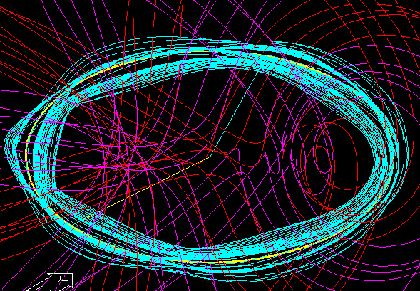
Graph 1 . Magnetic surface and axis (in yellow) for m=5
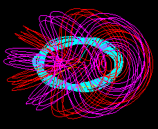
Graph 2 . Perpective of filamentary coils for m=5.
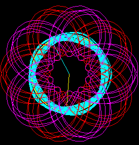
Graph 3 . Layout for m=5

Graph 4 . Layout for m=3 and magnetic axis in yellow
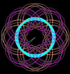
Graph 5 . Ground plan for m=4 with magnetic surface and magnetic axis
Last Update 4-1-2006